Big-O notation is used in computer science to describe the performance or efficiency of algorithms in terms of their growth rate related to the input size. It describes how the number of operations for an algorithm gets bigger as the number of processed elements increases, providing a way to analyze and compare the efficiency of algorithms in terms of their scalability. Here’s a cheat sheet that illustrates Big-O and its various runtime behavioral variants.

Big-O at a glance Algorithms Matrix O(1) - Constant Time O(log n) - Logarithmic Time O(n) - Linear Time O(n log n) - Linearithmic Time O(n^2) - Quadratic Time O(n^c) - Polynomial Time O(2^n) - Exponential Time O(n!) - Factorial Time Summary

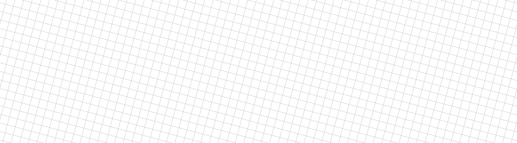
Big-O at a glance

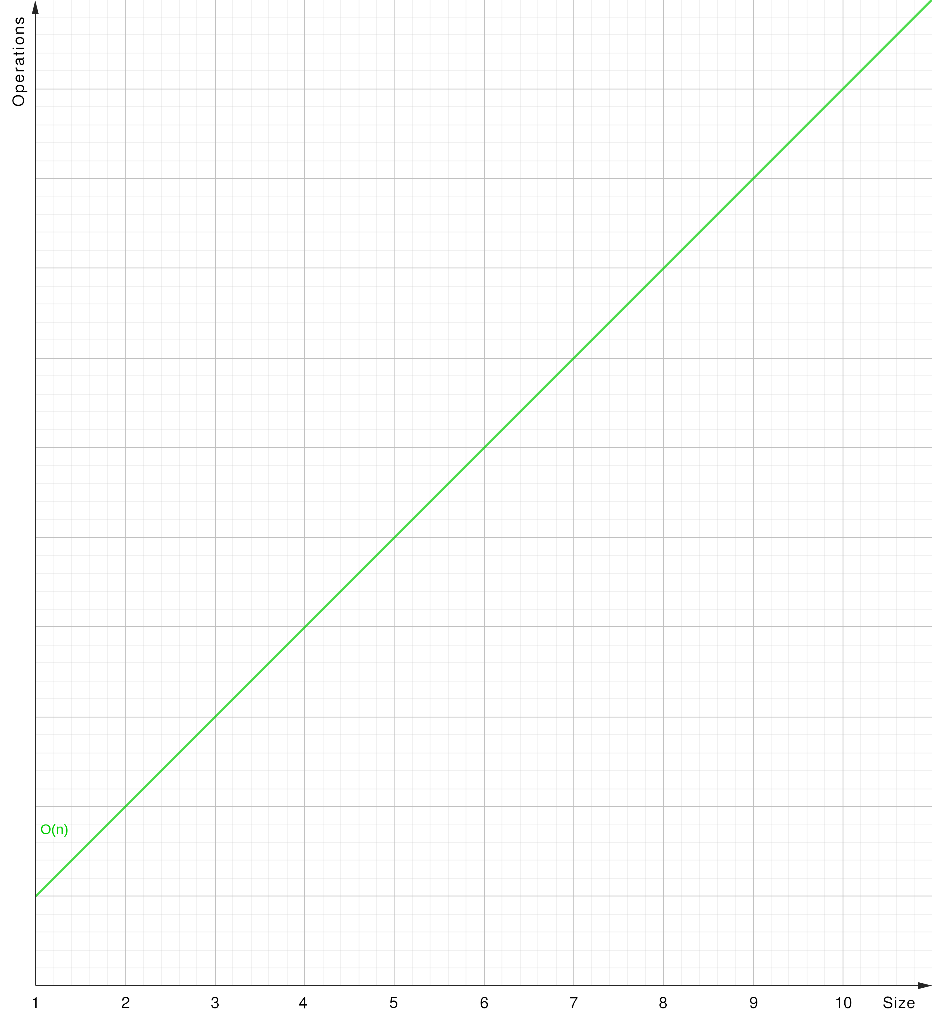
The graphs denote the increase of effort (operations) in relation to the requested size (of elements to be processed) for the various Big-O notations. Play around with the graphs using GeoGebra graphing calculator!¹

In the long term the proposition O(1) < O(log n) < O(n) < O(n log n) < O(n^2) < O(n^c) < O(2^n) < O(n!) is applicable

Algorithms Matrix

The table provides an overview of common algorithms and their according Big-O behavior.

	O(1)	O(log n)	O(n)	O(n log n)	O(n^2)	O(n^c)	O(2^n)	O(n!)
Indexed array	X
Binary Search		X
Linear Search			X
Array traversing			X
Breadth-First Search			X
Depth-First Search			X
Hash Table (average/worst)	X		X
Merge Sort				X
Quick Sort				X
Heap Sort				X
Nested Loop					X
2D arrays					X
Bubble Sort					X
Selection Sort					X
Insertion Sort					X
Triple Nested Loops						X
Brute-Force							X
Factorial (Permutation)								X

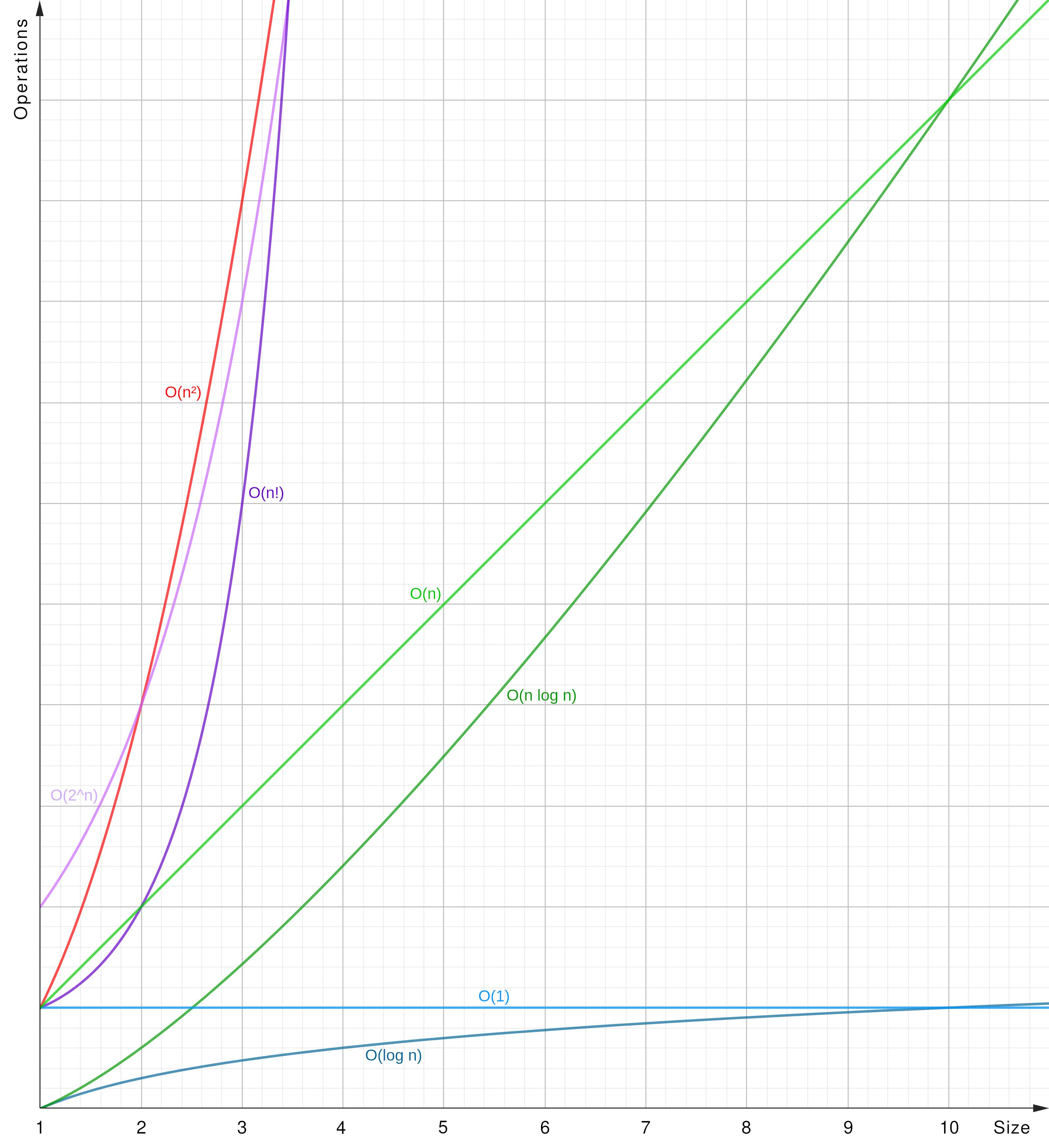
O(1) - Constant Time

O(1): The algorithm’s runtime is constant, irrespective of the input size (y = 1).

O(1)

Indexed array: Accessing an element in an array by index, regardless of the array size.
Hash Table (average): A dictionary using hash codes to look up keys and an according key buckets’ values.

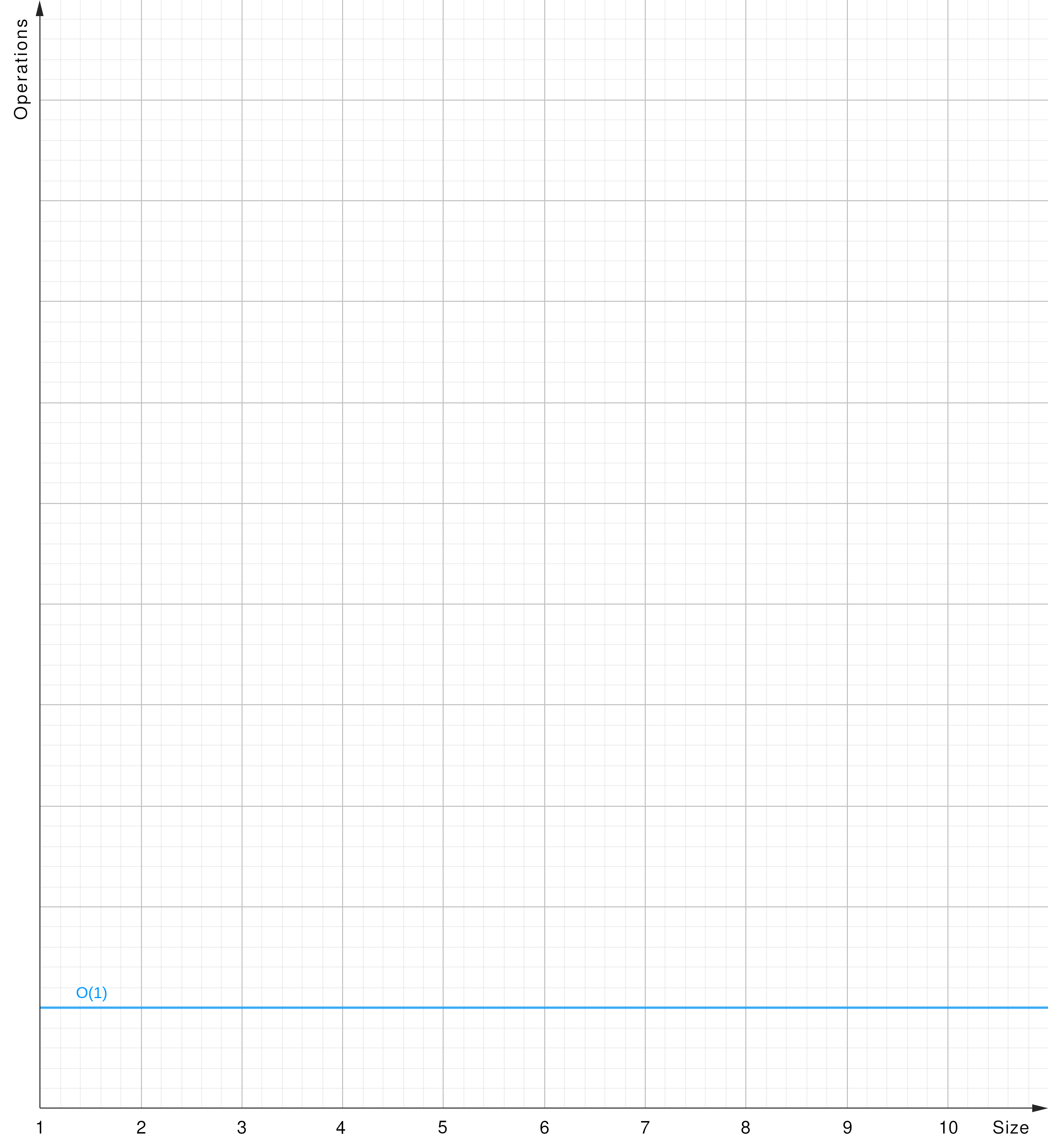
O(log n) - Logarithmic Time

O(log n): The algorithm’s runtime grows logarithmically relative to the input size (y = log x).

O(log n)

Binary Search: Binary search in a sorted array, where the search space decreases by half with each iteration.

O(n) - Linear Time

O(n): The algorithm’s runtime grows linearly in proportion to the input size (y = x).

O(n)

Array traversing: Iterating through an array or a linked list till encountering a specific element.
Linear search: Finding an element within a list sequentially checking each element for a match.
Hash Table (worst): A dictionary using hash codes to look up keys and an according key buckets’ values.
Breadth-First Search (BFS): Finding an element by searching a tree data structure, progressing horizontically first.
Depth-First Search (DFS): Finding an element by searching a tree data structure, progressing vertically first.

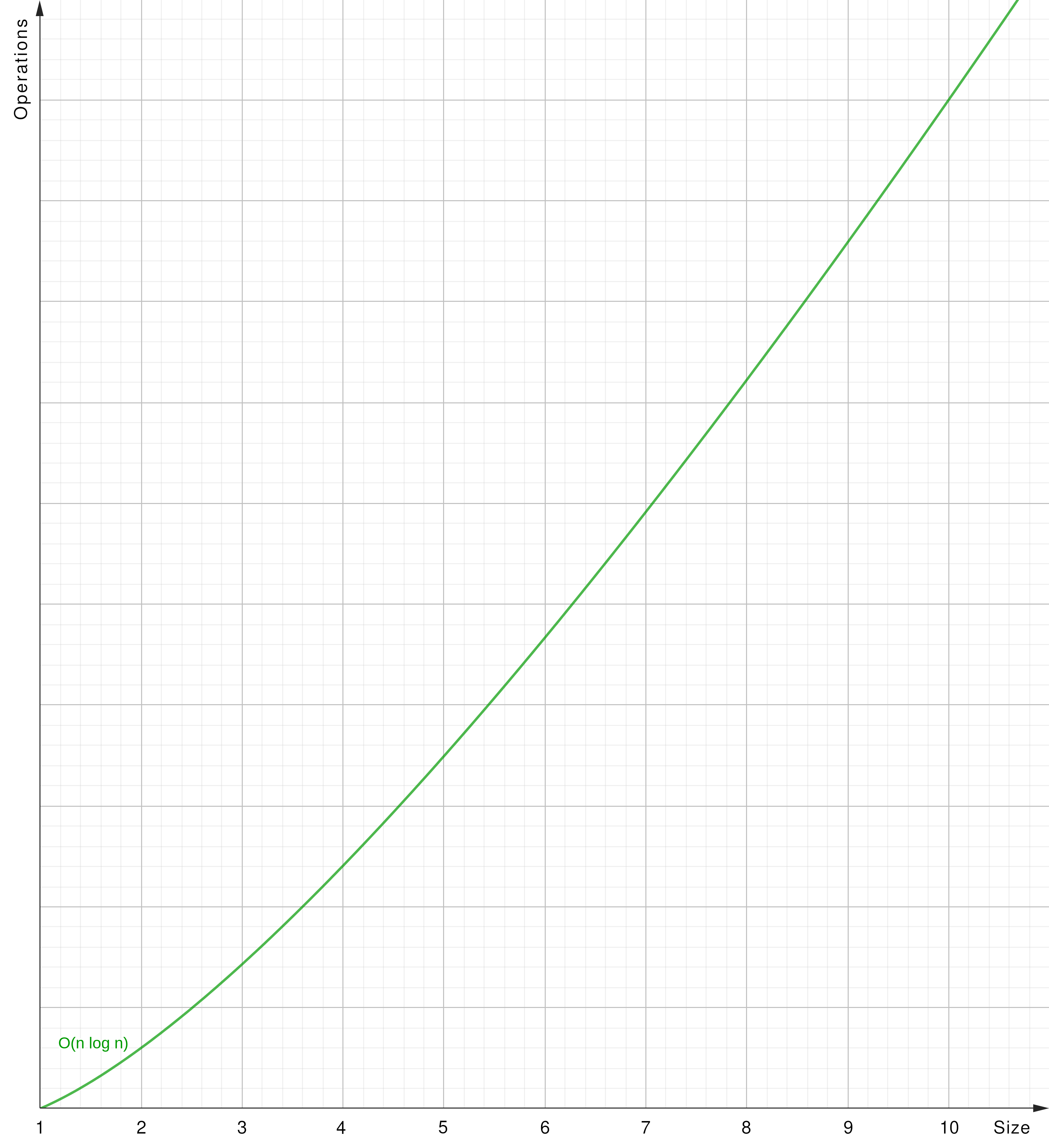
O(n log n) - Linearithmic Time

O(n log n): The algorithm’s runtime grows in a factor of n times log n concerning the input size (y = x log x).

O(n log n)

Merge Sort: Efficient general-purpose sorting algorithm.
Quick Sort: Efficient general-purpose sorting algorithm.
Heap Sort: Optimized sorting algorithm stepping through a list.

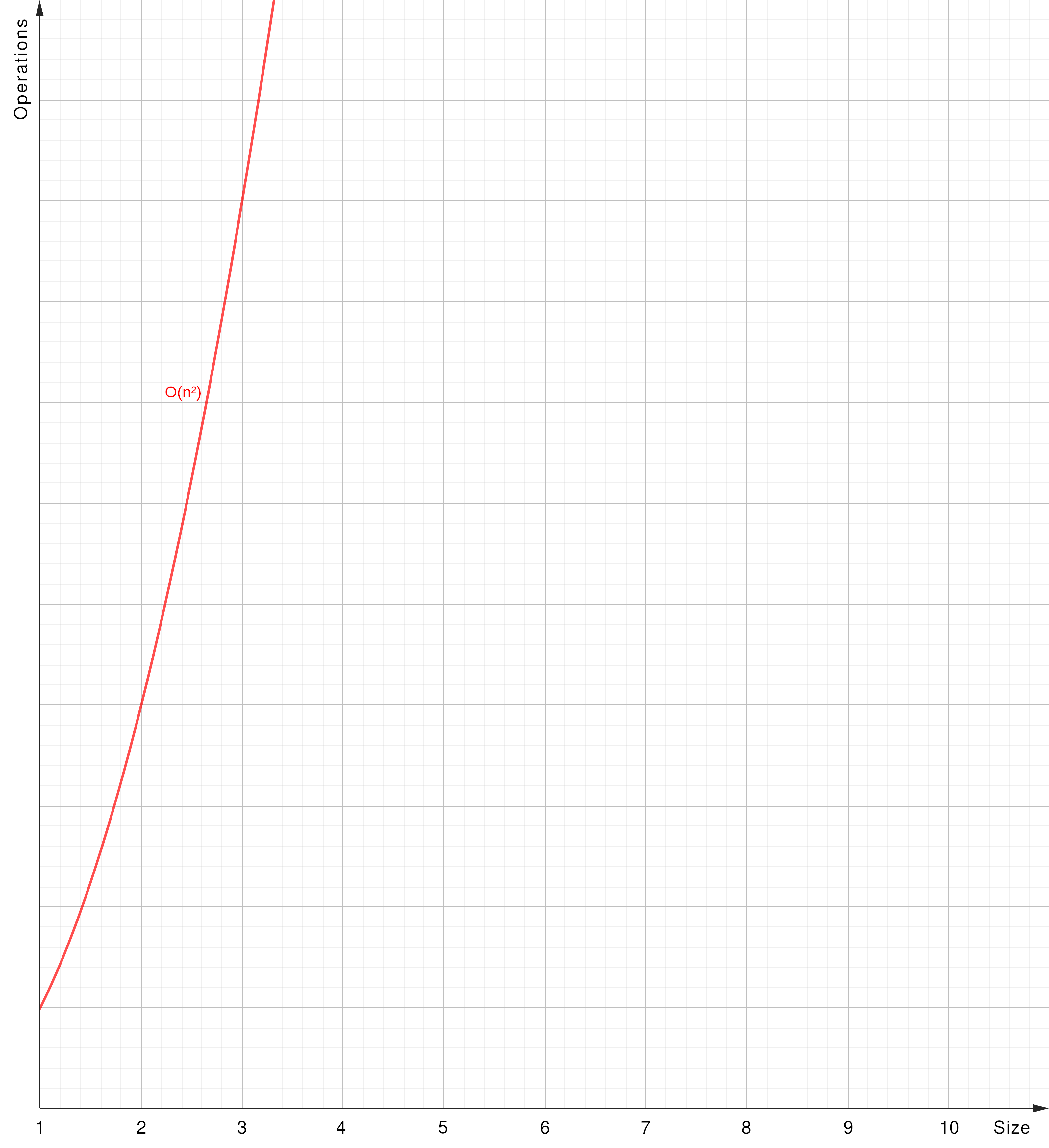
O(n^2) - Quadratic Time

O(n²): The algorithm’s runtime grows proportionally to the square of the input size (y = x²).

O(n²)

Nested Loop: Nested loop iterating through the same collection.
2D arrays: Looping through a 2D array with x-loop having a nested y loop.
Bubble Sort: Simple sorting algorithm repeatedly stepping through the list’s elements.
Insertion Sort Sort: Simple sorting algorithm repeatedly stepping through a list.
Selection Sort: Simple sorting algorithm repeatedly stepping through a list.

O(n^c) - Polynomial Time

O(n^c): The algorithm’s runtime grows as a polynomial function of the input size (y = x ^ c).

O(n^c) for n², n³, n⁴ and n⁵

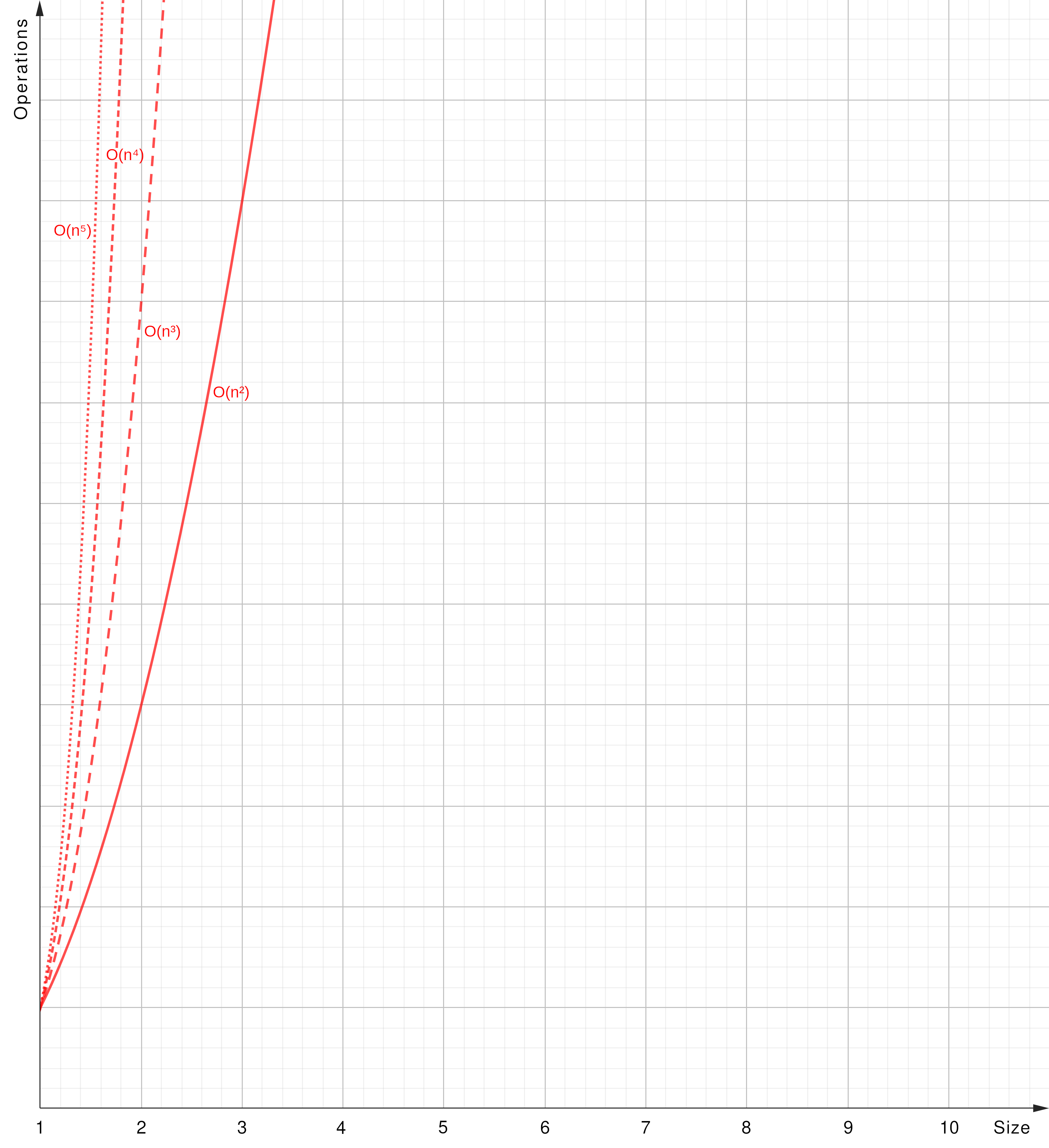Triple Nested Loops: Algorithms with three nested loops would have O(n^3), and so on.

O(2^n) - Exponential Time

O(2^n): The algorithm’s runtime grows exponentially concerning the input size (y = 2 ^ x).

O(2^n)

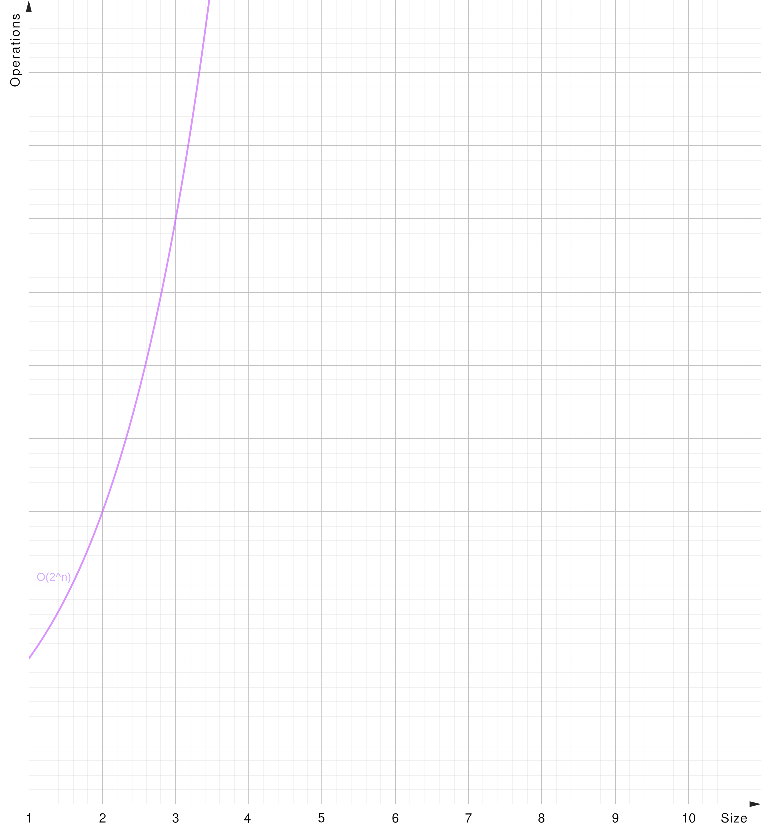Brute-Force: Brute-force or exhaustive search algorithms systematically checking all problem’s possiblities.

O(n!) - Factorial Time

O(n!): The algorithm’s runtime grows in factorial order concerning the input size (y = x!).

O(n!)

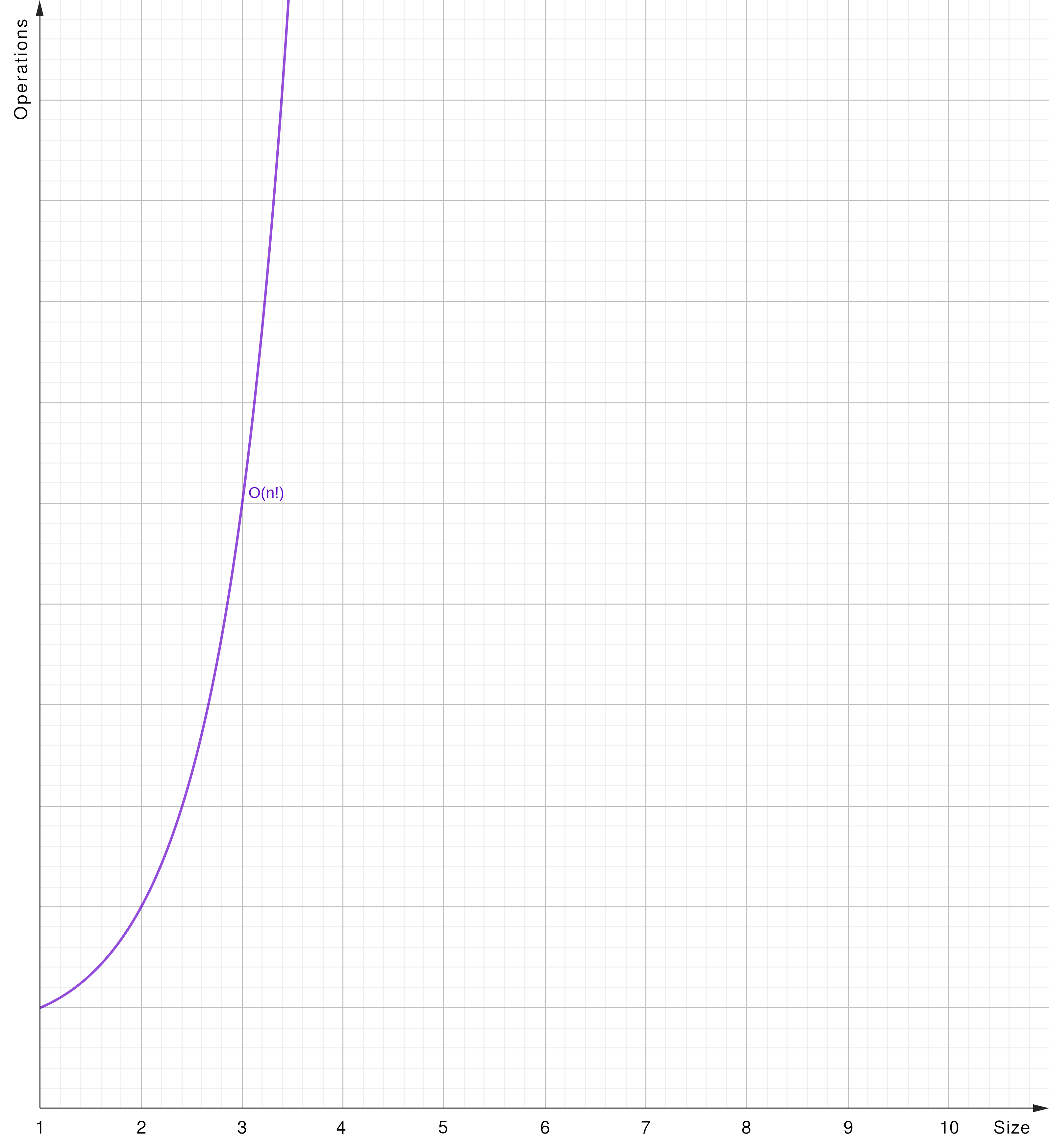Factorial (Permutation): Permutation or combination-based algorithms processing all combinations a particular list can be arranged to.

Summary

Keep in mind that Big-O notation describes the upper bound of an algorithm’s performance and might not represent the exact runtime in all cases. It helps in understanding an algorithm’s scalability and efficiency relative to input size.

Best to Worst (Efficiency)

In the long term the proposition O(1) < O(log n) < O(n) < O(n log n) < O(n^2) < O(n^c) < O(2^n) < O(n!) is applicable!

Generally, striving for algorithms with lower Big-O complexities leads to more efficient solutions for larger inputs.

Directly download the the “Big-O all graphs” project file to be used with the GeoGebra Graphing Calculator. ↩

Yet another Big-O cheat sheet

Categories

Tags